Let’s have a look at natural graph networks, introduced by Pim de Han et al. in their eponymous 2020 paper. We will take a direct and intuitive approach, circumventing the heavy duty mathematics from the original paper wherever possible!
Why do we want NGNs?
In standard graph convolutional network (GCN) a point p aggregates messages over all its neighbouring nodes q, in the following fashion:
\(\ v_p' = k_s v_p + \sum_q k v_q\)
Where v is the respective feature vector of the node and k is a weight matrix. The feature vector of the node itself vₚ is weighted with kₛ (where “s” stands for “self”). Notably there is no way for p to differentiate from which neighbouring node a given message came. The aggregation mechanism can only treat the message vₚ from the node itself and differently from incoming messages, using weights kₛ instead of k. Another way of saying this is that the way messages are aggregated is invariant under arbitrary permutations of its neighbours.
Permutation: from Latin permutare ‘change completely’. Permutation is just another word for swapping. In this case we mean swapping the features of two (or more) different nodes.
Invariant: literally ‘no change’.
If a function, say a neural net (NN) is invariant under some transformation, it means that the output does not change if we apply the transformation to the input.
Illustrated in this diagram is a NN that recognises cats and is invariant under scaling. Whether the cat was scaled down or not, the output does not change.
In contrast, in convolutional neural networks (CNNs) we have a kernel (usually 3x3), where each value in the kernel is a free parameter. In our GCN this would correspond to a point p on the grid having different weight matrices kᵢ for each of its eight neighbours and one for itself.
\(v_p' = \sum_{i \leq 9} k_{i} v_{i}\)
Using a GCN instead of a CNN on a pixel grid would reduce its kernels to blob filters, ie. a filter in which all values except that in the centre (kₛ) are equal.
An additional feature of CNNs is that each point on the grid is treated the same. Whether a car is in the upper right corner or in the left does not matter, the neuron corresponding to recognising cars it will light up in the appropriate location on the next layer. This is also called equivariance under translation.
Equivariant: literally ‘same change’. Closely related to invariant, equivariant means that instead of no change there is the same, or proportional change in the output.
In this diagram we can see an example where a cat is scaled down and then processed by a NN that is scale equivariant. The cat can ei ther be first scaled and then classified or classified and then scaled, both yield the same result, i.e. they commute. This commutation relation is the essence of equivariance. Also note that the transformations are not necessarily equal. Shrinking the cat does not result in a shrinking of the word ’cat’. The equivalent change in the output is the addition of ’small’.
This equivariance under translation enables the CNN to share weights across the whole pixel grid, so that recognising a car in two different corners can be reduced to one problem instead of being learned in every separate point on the grid.
Conversely this also is only makes sense if the data itself possesses a certain symmetry. Images lend themselves to this because pixel grids tend to posses translational equivariance; similar pixels represent similar objects no matter where on the pixel grid they are. In general, the symmetries in the NN should try to mirror the symmetries of the problem it is solving.
Generalising CNNs
So, inspired by CNNs we wish to generalise certain features to more general graphs than grids:
more expressive kernels than blob filters (invariance under permutation of neighbours)
equivariance under symmetries for weight sharing
Now we have to consider when sharing weights between to nodes is sensible. As an example, lets look at graph categorisation for a set of small graphs.
If two graphs are indistinguishable from another in structure we call them isomorphic.
Isomorphism: from Greek ‘same shape’.
\(\begin{equation*}
\psi: G \to G'
\end{equation*}\)
An isomorphism is a mapping of nodes of one graph G, onto graph G′ such that all the edges of the graph are preserved. That means if p and q share an edge in G and are mapped to nodes p′ and q′ in G′, p′ and q′ must be connected as well. The converse holds for p and q not sharing an edge. Depicted below, are three graphs, of which only the two on the left are isomorphic.
It is only natural that two indistinguishable graphs should be treated the same. In fact this is where the paper derives its name from. Naturality codifies precisely this idea of identical treatment of identical graphs. In more mathematical terms we ask that graph isomorphisms and our network commute with each other. From this commutation relation we will derive all conditions our network must full fill.
Back to our set of small graphs: Assume we first divide our set of graphs into subsets of isomorphic graphs, via some algorithm. Then we train a different multi layer perceptron (MLP) or just a different weight matrix on each of these subsets. We could then assume that we fulfilled our naturality condition, that the same features on the same graph will always result in the same output. But we are still missing something!
Automorphism: derived from joining ’auto’ and ’isomorphism’: self similar a.k.a. symmetric.
\(\begin{equation*}
\phi: G \to G
\end{equation*}\)
A graph G is said to posses an automorphism if there exists a permutation of nodes that preserves all edges. This can be formulated as an isomorphism mapping a graph to itself. If there exists such a permutation beyond trivially mapping each node to itself, it is also referred to as a symmetry.
Let’s take a look at an example graph and find a few automorphisms on it:
Up until now we hadn't considered this. The output of our NN might have depended arbitrarily on which way we applied it to a graph because it fit onto the graph in multiple ways due to its symmetries. That would mean that there existed isomorphisms, namely automorphisms, which did not commute with our NN!
To solve this we will examine each of our isomorphic classes for automorphisms and constrain our NN to be equivariant under these symmetries. Additionally this results in a reduction of parameters, which if our data had this symmetry were superfluous to begin with.
So, if we follow these steps:
Find isomorphic classes ⇒ Share weights for each class
Find automorphisms ⇒ Constrain weights to be equivariant under these
the paper proves that we will find a global natural graph network (GNGN), that will commute with all isomorphism.
Naturality, but Local
But what if the graphs are not small and we only have a few, maybe even only one huge graph like a social network? Then this approach becomes infeasible. Iso- and automorphisms becomes increasingly unlikely the more nodes and edges we have, and finding them becomes intractable. What we want is some local way to apply the same principles.
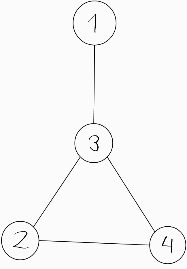
We will illustrate all the process on this simple graph. The node features will only be scalars (1,3,2,4) for ease of understanding, but of course this generalises to feature vectors.
Our local natural graph network (LNGN) will work by passing messages, analogously to a GCN. The difference will be that these messages are passed from neighbourhood to neighbourhood instead of from point to point.
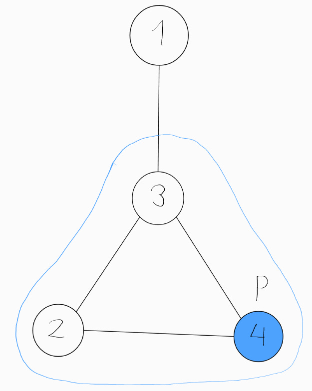
Neighbourhood: The neighbourhood Gₚ of p element G, is a subgraph of G, containing p. We will include all nodes sharing an edge with p and all edges between them. For example, the neighbourhood of node p is circled in blue.
We will associate each neighbourhood with a vector containing all features of its nodes. This will be called its representation. Isomorphisms, automorphisms, and our weights will also have representations, which we will introduce as they come up.
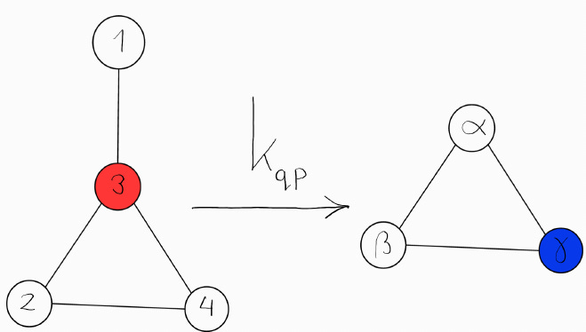
In our example we will consider the message being sent along edge_{qp}, marked here with a very small arrow.
Here the neighbourbourhoods of q and p are circled in red and blue respectively. The edge between them is also marked by an arrow labeled k_{pq}.
The message is sent from the neighbourhood of q (circled in red) to the neighbourhood of p (circled in blue).
For clarity here is another figure, showing the same message being passed via weights k_{qp}, from p’s to q’s neighbourhood:
We can also express this as a matrix multiplication, where k_{qp} is a 4x3 matrix:
k_{qp} is dependent on both the neighbourhood of p and of q. The union of these two neighbourhoods, including the marked, directional edge from q to p is also called the neighbourhood of edge_{qp}.
Since we our weights/kernel are identified with the edge, this is also how we will our find isomorphic subgraphs for weight sharing. We will share weights between two edges if their neighbourhoods are isomorphic.
Intuitively, we share weights because if the two edges neighbourhoods are identical i.e. isomorphic (and thus the neighbourhoods of start and target node) it is only natural that they we treat messages being passed through those edges the same way. Another way to phrase this, is that swapping the message being passed through two isomorphic edges, and applying the weights of that edge k_{qp} must commute. That is k_{qp} must be equivariant under edge neighbourhood isomorphisms.
Automorphism Constraints
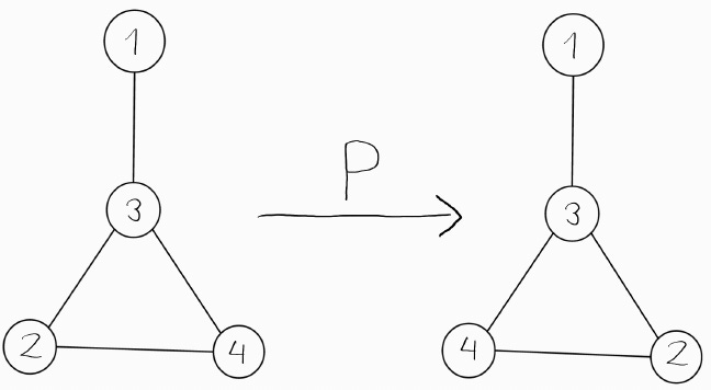
So, we covered weight sharing due to isomorphisms. What about the constraints we got on GNGNs due to automorphisms? This carries over as well. Automorphisms, that is permutations of nodes, that preserve the edges, can be represented by permutation matrices. So, when the automorphisms swaps two nodes, the permutation matrix swaps those two entries when applied to the neighbourhoods feature vector.
Let us find the automorphism in our example and see what permutation matrix it is represented as for our choice of feature vectors.
As you can see, when we multiply the feature vectors by the permutations, they swap exactly the entries we would expect.
Our naturality requirement remains unchanged, so let's illustrate what this means for out k_{qp}. If we permute two entries in the input vector and the two corresponding nodes are also part of the target node p's neighbourhood, and therefore the feature vector vq, then these two entries must also be swapped. The representations of the two permutations are different in general, but represent the same action (the automorphic permutation) on the graph.
From this we get the following condition:
\(\begin{aligned}
k_{qp} P v_q &= v'_p \\
P' k_{qp} v_q &= v'_p \\
\implies k_{qp} P v_q &= P' k_{qp} v_q \end{aligned}\)
And since this must hold for any vq:
\(k_{qp} P = P' k_{qp}\)
This is the constraint for weight matrix k_{qp} that the automorphism gives rise to. Now, we can fill our k_{qp} matrix with parameters, and write down the commutation relation explicitly.
\(\begin{bmatrix}
1 & 0 & 0 \\
0 & 0 & 1 \\
0 & 1 & 0
\end{bmatrix}
\begin{bmatrix}
a & b & c & d \\
e & f & g & h \\
i & j & k & l
\end{bmatrix}
=
\begin{bmatrix}
a & b & c & d \\
e & f & g & h \\
i & j & k & l
\end{bmatrix}
\begin{bmatrix}
1 & 0 & 0 & 0 \\
0 & 0 & 0 & 1 \\
0 & 0 & 1 & 0 \\
0 & 1 & 0 & 0
\end{bmatrix}\)
\(\begin{bmatrix}
a & b & c & d \\
i & j & k & l \\
e & f & g & h
\end{bmatrix}
=
\begin{bmatrix}
a & d & c & b \\
e & h & g & f \\
i & l & k & j
\end{bmatrix}\)
If these two matrices must be equal, then their elements must equal each other as well. Comparing elements we get the following constraints:
\(d=b, e=i, k=g, h=j, f=l\)
Inserting the parameters that are still free, we get:
\(k_{qp} =
\begin{bmatrix}
a & b & c & b \\
e & h & g & f \\
e & f & g & h
\end{bmatrix}\)
This is the most general matrix that satisfies our commutation constraint. For the sake of our model we can also decompose this k_{qp} into a linear combination of binary matrices:
These matrices form a basis for the constrained solution space, and our the remaining free parameters will be there parameters our model will learn. The kernel will be a linear combination of these basis matrices.
Algorithm
In summary our Algorithm consists of the following steps:
Preparation
Identify edge neighbourhoods
Sort edge neighbourhoods into isomorphic classes
Find automorphisms in said classes
Solve automorphism constraints
Training
Calculate kernel from parameters
Transport kernel to isomorphic neighbourhoods
Calculate message
Aggregate (e.g. sum) over all neighbours messages
What does this all mean?
What we have achieved, is a freamework that satisfies naturality, i.e. that isomorphic graphs be treated the same. In fact, the paper goes on to prove that LGNGs fullfill the naturality condition globally.
We originally set out to generalise the pleasing properties of CNNs to graphs. And if we apply LNGNs to a rectangular grid graph with diagonals added we recover a group equivariant CNN with 3x3 kernels! Why group equivariant? Because a grid not only has translational but also rotational and mirror symmetries.
Whether we want these additional equivariances, is a question that depends on our problem setting. If these symmetries were undesirable we could potentially mark edges or nodes to distinguish them. For instance if we did not want rotational equivariance in our CNN we could mark one of the edges per node as the “upward” edge.
In short we now have a tool to bake any symmetry our problem has into our GNN in a natural way!